Matrix boundaries
Return Loss
How a controlled boundary reduces the energy reflected back into the system.
Explore Return LossTHE PHYSICS OF QUIET / 03
Why wavelength, return paths and skin effect matter in a system that is never entirely free of high-frequency energy.
At audio frequencies, the dimensions of a cable, circuit board or listening room are usually very small compared with the wavelength of the musical signal. The usual circuit models work well.
The picture changes when unwanted energy reaches much higher frequencies. A cable or PCB track then becomes a path with length, geometry, a nearby return route and boundaries that can reflect energy.
This is a guide to physical principles, not a specification or a measurement of a particular Quiescent product.
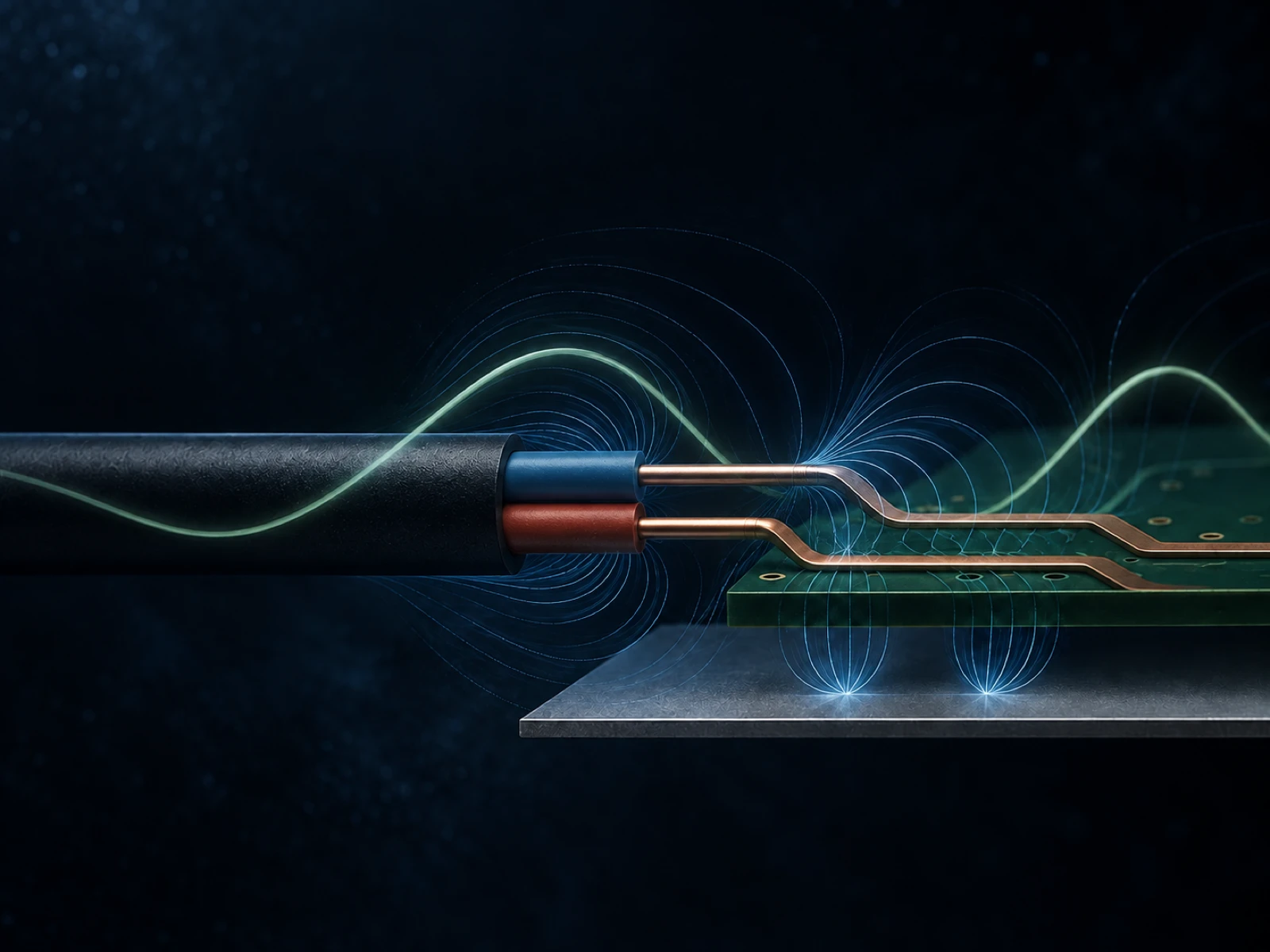
Audio-band programme material and high-frequency disturbance can occupy the same physical system, yet demand different levels of description. Neither picture cancels the other.
For a typical audio cable, a 20 kHz waveform is still kilometres long. A few metres of cable are therefore electrically short by comparison. At radio frequencies, the wavelength can approach the dimensions of a cable, a PCB trace, a connector or a gap in a reference plane. Energy can then propagate, couple and reflect in ways that a simple lumped-circuit sketch does not reveal.
The useful question is not whether audio equipment is secretly an RF system. It is whether high-frequency energy is present, and whether the paths available to it are controlled.
Illustrative scale model
A fixed 2 m cable and 100 mm PCB track are compared with the selected wavelength. The cable and PCB do not change; only the scale of the selected wave changes.
The example uses a propagation velocity of approximately 0.67c. Real cable and PCB velocity depends on dielectric and geometry. The motion is deliberately normalised to show spatial scale, not signal speed.
Notice that the wavelength is still vast compared with a cable or a board. This is why audio-band circuit models are normally appropriate.
As frequency rises, the same physical length occupies a meaningful part of a wavelength. Geometry and the return path begin to matter more.
At very high frequencies, a short PCB feature or connector can be a significant boundary. Discontinuities can couple or reflect energy.
Skin effect describes a change in current distribution within a conductor as frequency rises. The changing magnetic field associated with the current makes the inner part of the conductor a higher-impedance route, so more current density is found nearer the surface.
It is a real and useful effect. It is not, however, a story in which the audible bass is assigned to the core and the audible treble is assigned to a faster outer lane.
Skin depth becomes smaller as frequency rises. In copper, the approximate skin depth is about 0.47 mm at 20 kHz, 0.066 mm at 1 MHz, 0.0066 mm at 100 MHz and 0.00066 mm at 10 GHz. These values are guides: conductor material, magnetic permeability, temperature and shape also matter.
As the available depth becomes smaller, the effective conducting area is reduced and AC resistance rises. Nearby conductors can add a related effect, known as proximity effect, because each conductor changes the magnetic field seen by the other.
| Illustrative frequency | Approximate wavelength in a 0.67c cable | Approximate copper skin depth |
|---|---|---|
| 20 Hz | 10,000 km | 15 mm |
| 20 kHz | 10 km | 0.47 mm |
| 1 MHz | 200 m | 0.066 mm |
| 100 MHz | 2 m | 0.0066 mm |
| 10 GHz | 20 mm | 0.00066 mm |
These figures explain why a conductor can behave very differently for unwanted high-frequency energy than it does for the musical signal.
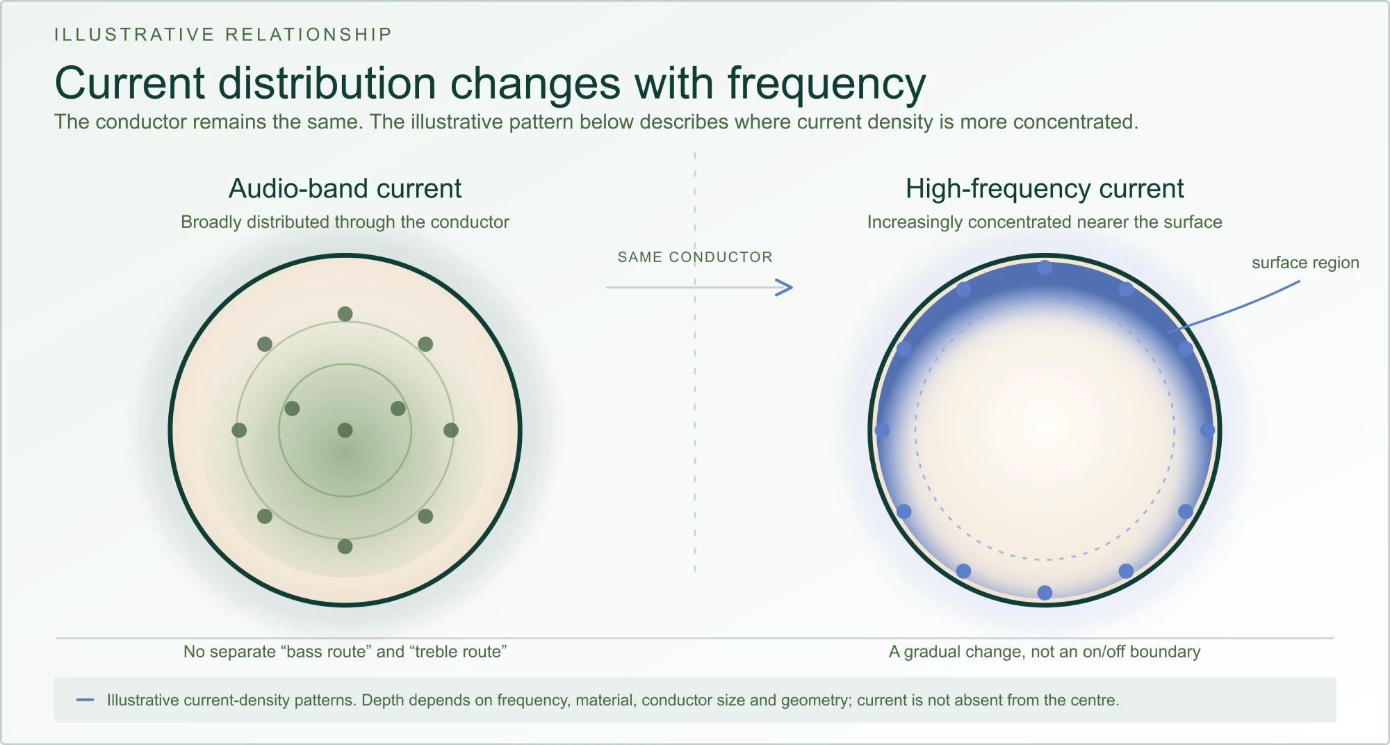
Skin effect is a frequency-dependent redistribution of current density. It does not divide an audio signal into separate bass and treble paths.
Myth: bass travels through the centre of a cable and treble travels around its outside, so the two arrive at different times.
Reality: music is a changing waveform made of frequency components. In a conventional audio cable, those components are not assigned separate routes or simple different travel speeds. Cable loss and phase can vary with frequency, but that is a circuit and transmission-path question—not evidence for a bass-versus-treble race through the conductor.
Myth: skin effect is either the explanation for every audible cable difference, or entirely irrelevant to audio.
Reality: at audio frequencies it is usually not a useful explanation for separate musical timing. Yet an audio system can contain, generate and receive energy far above the audio band. At those frequencies, skin effect is one part of a wider set of effects involving conductor geometry, dielectric loss, proximity, return paths and reflections.
Useful question: what high-frequency energy is present, where can it travel, and what does it encounter at each boundary?
A conventional stranded cable is normally used for flexibility. If its strands are electrically joined at the ends, it is still one conductor from the viewpoint of the circuit. Dividing the copper into visible strands does not, by itself, guarantee lower high-frequency resistance or controlled propagation.
Litz wire is a specific construction in which individually insulated strands are arranged to share their positions through the winding. It can reduce skin- and proximity-effect loss in appropriate frequency ranges, particularly in magnetic components. It is not a universal answer for an interconnect or a mains cable, and it introduces its own construction, capacitance and termination considerations.
For high-frequency behaviour, the whole geometry matters: conductor size and surface, spacing, dielectric, shield or reference plane, connector transitions and the route available for return current.
High-frequency energy does not automatically become audible simply because it is present. In a linear, well-isolated circuit it can remain outside the useful signal path and be rejected.
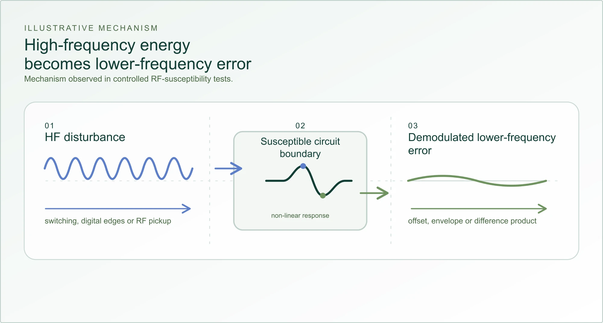
The situation changes if it reaches a non-linear, time-varying or insufficiently isolated circuit boundary: for example, a semiconductor junction, protection structure, input stage, switching device, reference or power path. At such a boundary, high-frequency energy can be rectified or mixed, producing an offset, envelope or difference product at a much lower frequency.
Controlled RF-susceptibility work on audio circuits demonstrates this mechanism. It does not mean that every installation will behave in the same way, or that every high-frequency source will be audible. It explains why controlling high-frequency paths before they reach a susceptible boundary is technically meaningful.
RF-immunity tests deliberately inject or radiate a defined high-frequency signal while observing the circuit output. When the carrier is amplitude-modulated, a susceptible non-linearity can recover the modulation as a lower-frequency disturbance. The sources in the final technical-notes Row include examples for audio circuitry and audio-power paths.
The useful conclusion is modest but important: an audio system is not defined only by its audio-band schematic. Its high-frequency environment, the routes through it and the boundaries it encounters can affect the conditions under which the musical signal is processed.
Skin effect tells us how current density redistributes within a conductor. It does not, by itself, tell us how unwanted high-frequency energy propagates through an installation. For that, the conductor, its nearby return route, the dielectric, the reference plane and the surrounding boundaries have to be considered together.
Field terminology gives us a compact way to describe those relationships. It need not turn the page into a microwave-engineering lesson; the purpose is to show why one visible wire is never the whole high-frequency path.
Imagine high-frequency energy travelling along the direction of a cable or track. In a TM (transverse magnetic) field pattern, the electric field has a component in that direction. This makes TM a useful simplified model for unwanted energy associated with a conductor surface and its surrounding environment.
In a TE (transverse electric) field pattern, the electric field is entirely across the direction of travel. It is a different relationship between the field and the surrounding structure. Neither term describes a separate lane for bass or treble; they are ways of describing high-frequency fields.
A deliberately designed cable or PCB track with a close, defined return is more accurately described as a quasi-TEM transmission path.
In the illustrative surface-related disturbance model used here, a TM-like field relationship is a useful way to describe one possible coupling path. Real cable and PCB structures are normally quasi-TEM and can contain mixed field behaviour determined by geometry, materials and boundaries.
Illustrative path model. At high frequency, the forward path, its return environment and nearby boundaries form one structure. A connector, branch, gap or plane discontinuity can alter that structure and create a place where energy couples or reflects. This is a teaching model, not a field simulation of a particular product or installation.
Matrix is Quiescent’s engineered absorptive environment for unwanted high-frequency energy. It is not an audio-band equaliser, and it does not assign different musical frequencies to separate paths through a conductor.
Its purpose is to manage high-frequency propagation, reflection and coupling across the relevant field-and-boundary structures, so less unwanted energy remains available to reach a susceptible circuit boundary. That approach recognises both surface-related and surrounding-field behaviour without reducing the system to one visible cable or one central treatment point.
Power, grounding, interconnects, speaker connections, circuit boards and components can all form part of the same high-frequency environment. The result in any installation depends on its equipment, geometry, connections and disturbance conditions; the principle is to reduce the opportunity for unwanted energy to become lower-frequency error.
The question is not whether high-frequency energy exists. It is whether the system gives it uncontrolled paths to travel, reflect and interact with susceptible circuitry.
Controlled RF work explains why such interaction can create lower-frequency error. Wavelength, skin effect and field structure explain how the energy can travel. Matrix is Quiescent’s systems-level response: manage the path before that unwanted interaction has the opportunity to occur.
Explore the wider system view of unwanted energy, controlled boundaries and the paths that connect an audio installation.
Matrix boundaries
How a controlled boundary reduces the energy reflected back into the system.
Explore Return LossMatrix boundary
How a Matrix boundary reduces unwanted energy that would otherwise pass through and continue onward.
Explore Insertion LossMains and earth
A systems view of balanced supply, transformer coupling and the high-frequency behaviour of earth paths.
Explore Balanced MainsThis page is a conceptual guide to wavelength, conductor loss, field descriptions and propagation. It does not model a particular cable, PCB, product or installation. Skin depth, impedance, propagation velocity, coupling and susceptibility depend on material, geometry, dielectric, frequency and the surrounding return structure.
The RF-susceptibility references below show controlled mechanisms, not a measured outcome for an individual audio system. TE, TM and quasi-TEM are field descriptions whose usefulness depends on the physical geometry being considered.