Matrix boundaries
Return Loss
How a controlled boundary reduces the energy reflected back into the system.
Explore Return LossTHE PHYSICS OF QUIET / 05
How a Matrix Boundary reduces the unwanted high-frequency energy that reaches a protected part of an audio system.
An audio system is a connected electrical environment. Unwanted high-frequency energy can travel along power, grounding, chassis and interconnect paths, reaching parts of the system we would rather keep quiet. Insertion Loss gives us a way to describe how much of that energy is reduced as it passes through a treatment point.
Where Return Loss describes what comes back from a boundary, Insertion Loss describes what continues beyond it. This page follows the energy that attempts to cross a Matrix Boundary and enter a protected area.
A note on the model: the animation isolates Insertion Loss by holding reflection constant. It illustrates the principle rather than a measured product response.

The image is deliberately not a harbour wall. A hard wall sends a wave back and is useful when explaining reflection. A shallow beach gives an incoming wave a long, changing route over which it can lose energy. The lagoon beyond the beach is calmer because less of the incoming wave reaches it.
Insertion Loss is therefore about transmission. At 0 dB, the illustrative incoming wave crosses the Matrix Boundary without attenuation. As Insertion Loss increases, less unwanted energy reaches the protected area.
Return Loss and Insertion Loss are complementary, not interchangeable. Return Loss describes energy reflected back at a boundary. Insertion Loss describes energy transmitted through it. In the animation below, Return Loss is held at 20 dB so the small reflected wave stays constant while the transmitted wave changes.
How to read the graphic: the blue incident wave approaches from the external field. The narrow green reflected trace is deliberately held constant at 20 dB Return Loss. Beyond the Matrix Boundary, the dark transmitted wave shows the energy entering the protected area. Changing Insertion Loss changes that transmitted wave and its two readouts only.
The control changes only the illustrative Matrix Insertion Loss. The incident wave remains the same. Matrix Return Loss remains fixed at 20 dB. This makes the relationship clear: the changing quantity is the energy that crosses the boundary into the protected area.
Insertion Loss is stated in decibels, so the change is logarithmic rather than linear. A 3 dB Insertion Loss leaves about half the illustrative power to continue. At 10 dB, one tenth remains. At 20 dB, one hundredth remains. The animation shows both transmitted power and transmitted amplitude because they describe different aspects of the same wave.
At 0 dB, the transmitted wave continues at the same illustrative amplitude as the incident wave. As the selected value rises, the transmitted trace becomes progressively smaller. At 30 dB, the model leaves only 0.1% of the incident power and about 3.2% of the incident amplitude beyond the Matrix Boundary.
At 0 dB there is no illustrative Insertion Loss. The incident wave crosses the Matrix Boundary and enters the protected area at full amplitude. This is the useful starting comparison, not the desired outcome.
Move through 3, 6, 10, 20 and 30 dB. The incident wave and the small fixed reflection do not change. Watch only the transmitted wave beyond the Matrix Boundary become smaller.
The component reports both ratios. At 10 dB, 10% of the illustrative power crosses the boundary, while the transmitted voltage-amplitude ratio is about 31.6%.
The lagoon is an analogy, not a literal electrical model. In engineering terms, Insertion Loss compares the power that arrives at a treatment point with the power that emerges beyond it. The central question is simple: how much of the unwanted high-frequency energy is allowed to continue into the part of the system we are trying to protect?
For this illustration, Insertion Loss compares incident power with the power transmitted beyond the Matrix Boundary, expressed in decibels:
Insertion Loss = −10 log10(transmitted power ÷ incident power)
Higher Insertion Loss therefore means less transmitted power. The amplitude ratio is the square root of the power ratio, so it changes at half the decibel rate. The table uses the same relationship as the component above.
| Illustrative Insertion Loss | Transmitted power | Transmitted amplitude |
|---|---|---|
| 0 dB — no loss | 100% | 100% |
| 3 dB | About 50% | About 71% |
| 6 dB | About 25% | About 50% |
| 10 dB | 10% | About 32% |
| 20 dB | 1% | 10% |
| 30 dB | 0.1% | About 3.2% |
Exact behaviour depends on the device, cable and installation
The graph shows the frequency-selective design objective: preserve audio-band transmission while increasingly attenuating unwanted high-frequency energy.
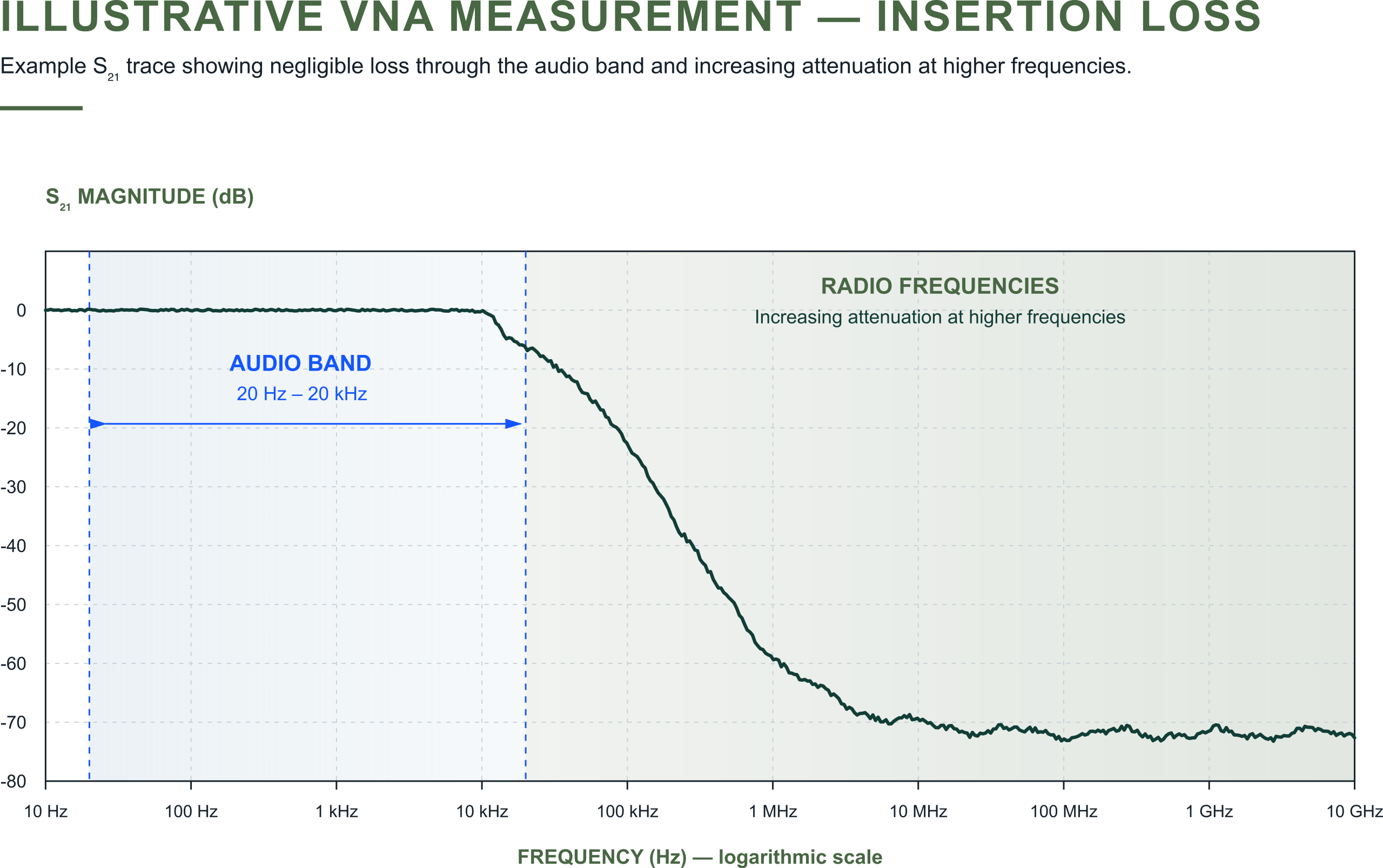
Illustrative frequency response, not measured product data.
At conventional audio frequencies, many system connections can often be treated as straightforward circuit paths. As frequency rises, the electrical route becomes more significant. Cable geometry, connector interfaces, chassis structures, component parasitics, and the paths shared by power and grounding can all influence where unwanted energy travels.
High-frequency energy moves through a connected environment. Its route depends on the geometry, impedances and boundaries it encounters. The protected area represents the part of that environment where Matrix reduces incoming unwanted energy.
The engineering task is frequency-selective: attenuate unwanted high-frequency energy while preserving the system’s intended audio-band behaviour.
A Matrix Boundary controls both transmission and reflection. Insertion Loss describes the reduction in unwanted energy passing into the protected area. Return Loss describes how little is reflected back into the wider system.
This page holds Matrix Return Loss at 20 dB to concentrate on transmission. The companion Return Loss in Audio Systems page holds the transmission question aside and makes the reflected field visible. Together, the two models describe a more considered route for unwanted energy than a simple hard barrier.
Quiescent uses these complementary controls to reduce unwanted high-frequency energy entering sensitive regions and returning through the wider system, while preserving the musical signal.
Music asks an audio system to preserve relationships of level, timing and harmonic structure as they change moment by moment. Reducing unwanted energy entering sensitive circuitry helps stabilise the conditions in which that signal is processed.
During our development and listening evaluations, reducing unwanted disturbance has repeatedly produced a clearer, more stable musical presentation.
The relevant paths and the extent of the improvement depend on the installation. The related Tracking Error in Audio Systems page illustrates how changing operating conditions can affect signal tracking.
Matrix boundaries
How a controlled boundary reduces the energy reflected back into the system.
Explore Return LossSystem application
How two Matrix boundaries can define a quieter environment around a sensitive part of a system.
Explore Audio Subsystem ProtectionSignal behaviour
How a changing disturbance environment can make it harder for a system to follow the musical signal precisely.
Explore Tracking ErrorThe animation and frequency-response graph are conceptual illustrations. Insertion Loss describes reduced transmission through a path or component, expressed in decibels. A practical measurement specifies the frequency range, reference condition, source and load impedances, and relevant return paths.
The references explain the underlying measurement and high-frequency principles. Quiescent’s own research and development informs their application to working audio systems.