Matrix boundaries
Insertion Loss
How a boundary reduces unwanted energy that would otherwise pass through and continue onward.
Explore Insertion LossTHE PHYSICS OF QUIET / 04
Why unwanted high-frequency energy can reflect, form standing-wave patterns, and be given a more controlled path away from the musical signal.
An audio system is more than a sequence of products. Its power, grounding, chassis and interconnect paths form one electrical environment. At higher frequencies, a change in impedance can cause part of an unwanted disturbance to turn back towards its source rather than continue onward.
Return Loss gives us a practical way to describe that reflection. A larger Return Loss number means less energy is returning. This page first makes the mechanism visible, then explains what the number means.
A note on the model: the animation isolates reflection at a boundary and shows how Return Loss changes the returning wave. It is a conceptual illustration, not measured product data.

The incoming wave carries energy towards the wall. When it reaches that boundary, not all of the energy continues on or disappears. Some is reflected back into the water.
The reflected wave then encounters waves still travelling towards the wall. Where they meet, they interact — sometimes reinforcing one another, sometimes opposing one another.
Something analogous can happen to high-frequency electrical energy. When a travelling disturbance encounters a change in impedance, some of its energy can be reflected back towards its source.
Counterintuitively, higher Return Loss means less energy comes back.
In an electrical system, a connector, termination, interface or change in construction can present a different impedance to a signal path that is electrically long at the frequency of interest. The travelling energy then does not all continue in one direction: part may be reflected.
The incident and reflected waves occupy the path at the same time. Their sum can create a pattern of fixed high and low points, known as a standing wave. The location and severity of those points depend on frequency, path length, propagation behaviour and the degree of mismatch.
Full reflection is a useful boundary case for learning. Real systems are more complex: reflections can be partial, frequency dependent and distributed across several paths. The underlying principle, however, is the same—less reflected energy means a less pronounced standing-wave pattern.
The animation separates the incident wave, the returning wave and their combined pattern. The two travelling waves move; the combined pattern makes the interference along the path visible.
The control changes only the illustrative Return Loss at the boundary. It recalculates the reflected wave and, with it, the combined standing-wave pattern. The incident wave is held constant so the changing reflection is easy to see.
Return Loss is stated in decibels, so the relationship is not linear. A 10 dB increase means ten times less reflected power; the reflected amplitude changes by the square root of the power ratio. The values beneath the animation show both, because they describe different aspects of the same reflection.
Full reflection is 0 dB Return Loss. All illustrative incident power returns from the boundary, creating the strongest combined pattern in this model.
Move through 3, 6, 10, 20 and 30 dB. The returning wave becomes smaller, and the variation in the combined pattern reduces with it.
The component shows reflected power and reflected amplitude separately. At 10 dB, for example, 10% of the illustrative power is reflected, while the returning voltage-amplitude ratio is about 31.6%.
The animation makes the mechanism visible. Return Loss provides the engineering shorthand: it compares the power travelling towards a boundary with the power reflected back from it.
Reducing reflection leaves less unwanted energy returning along the incoming path. Return Loss quantifies this boundary behaviour and helps us assess how high-frequency disturbance moves through the wider system.
Return Loss compares incident power with reflected power, expressed in decibels. The larger the Return Loss, the smaller the reflected portion. In power terms:
Return Loss = −10 log10(reflected power ÷ incident power)
This is why a 10 dB change is meaningful: every additional 10 dB reduces the reflected-power ratio by a factor of ten. The table uses the same relationship as the control above.
| Illustrative Return Loss | Reflected power | Reflected amplitude |
|---|---|---|
| 0 dB — full reflection | 100% | 100% |
| 3 dB | About 50% | About 71% |
| 6 dB | About 25% | About 50% |
| 10 dB | 10% | About 32% |
| 20 dB | 1% | 10% |
| 30 dB | 0.1% | About 3.2% |
Exact behaviour depends on the device, cable and installation
The design objective is to reduce reflection of unwanted high-frequency energy while preserving the system’s intended audio-band behaviour.
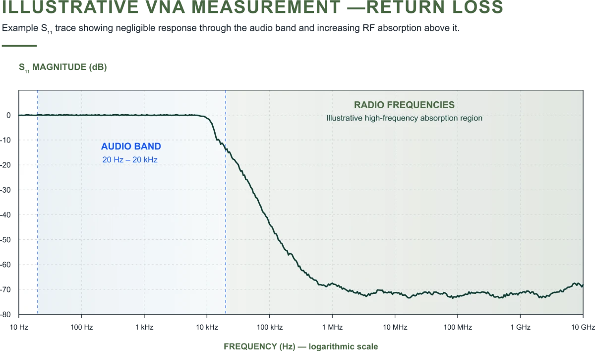
Illustrative frequency response, not measured product data.
At conventional audio frequencies, many interconnects and internal connections are short relative to wavelength and can often be treated as simple circuit connections. As frequency rises, the electrical length of a path becomes more significant. Cable geometry, impedance changes, connector interfaces, chassis structures and component parasitics can all influence how energy travels and returns.
High-frequency behaviour depends on the complete path: its geometry, impedances, return routes and boundaries. Assessing those relationships reveals where unwanted energy travels and where it is reflected.
This is also why conventional filtering and matching solve different problems. A capacitor, for example, is not an ideal component at all frequencies: parasitic inductance and self-resonance alter its behaviour. Good engineering considers the route, the boundary and the frequency range together.
Matrix manages unwanted high-frequency energy across the connected system. Return Loss describes the reflected portion at a boundary; Insertion Loss describes the reduction in transmission beyond it. Quiescent uses both to control where unwanted energy returns and where it continues.
An absorptive boundary reduces reflection while dissipating unwanted energy. Return Loss quantifies the reflection; assessing transmission alongside it helps establish the boundary’s overall behaviour.
The engineering aim is to stabilise conditions around the musical signal, helping the existing components preserve its level, timing and harmonic relationships.
Music asks a system to preserve changing relationships of level, timing and harmonic structure. Reducing unwanted energy circulating and returning through sensitive paths helps stabilise the conditions in which the signal is processed.
During our development and listening evaluations, reducing unwanted disturbance has repeatedly produced a clearer, more stable musical presentation.
This experience informs Quiescent’s approach to reflection and transmission control. The relevant paths and the extent of the improvement depend on the equipment, connections and disturbance conditions.
Matrix boundaries
How a boundary reduces unwanted energy that would otherwise pass through and continue onward.
Explore Insertion LossSystem application
How two Matrix boundaries can define a quieter environment around a sensitive part of a system.
Explore Audio Subsystem ProtectionSignal behaviour
How a changing disturbance environment can make it harder for a system to follow the musical signal precisely.
Explore Tracking ErrorThe animation and frequency-response graph are conceptual illustrations. Return Loss describes reflected power relative to incident power under defined conditions. Practical assessment specifies frequency, reference impedance, measurement plane and the connected paths.
The references explain the underlying wave and component principles. Quiescent’s research and development informs the application of these principles to working audio systems.