Circuit response
RF in Analogue Audio Circuits
How RF can couple into an analogue circuit and become a lower-frequency error.
Explore RF in Analogue Audio CircuitsTHE PHYSICS OF QUIET / 10
Why watts matter, but do not by themselves describe how an amplifier controls a real loudspeaker.
A power amplifier is asked to deliver voltage and current into a load that changes with frequency, crossover behaviour and driver motion. The loudspeaker is part of the electrical system, not merely its destination.
This page connects established electroacoustic and electronic principles with Quiescent’s research into the amplifier, cable and loudspeaker as one working system.

Loudspeaker sensitivity describes the sound output produced by a specified electrical input under stated test conditions. Listening distance, the room and the peaks in music help determine how much output an amplifier needs to provide. A rated-power test into a fixed resistance offers a useful baseline, but a real loudspeaker is not a fixed resistance.
An 8-ohm or 4-ohm label is a starting point, not the full electrical picture. The load changes across the frequency range as the crossover and drivers operate. Two loudspeakers with the same nominal rating can therefore make quite different demands on an amplifier.
A loudspeaker’s impedance—its opposition to alternating current—changes with frequency. Where that impedance falls, maintaining the same output voltage calls for more current. How demanding that is depends on the listening level as well as the loudspeaker.
Voltage and current do not always peak at the same moment. This timing difference is called phase. When they are out of step, some energy is briefly stored and returned during each cycle, changing when the amplifier must handle current. A low-impedance region and a substantial phase shift can act together, but neither one alone proves that a loudspeaker is difficult to drive.
A moving-coil driver is both a motor and, as it moves, a generator. Current through the coil creates force. Movement of the coil through the magnetic field generates a voltage known as back EMF. In a simplified model, the driver’s electrical behaviour reflects the coil’s resistance, its inductance and this motion-generated voltage. The last of these follows how quickly the coil moves.
The moving mass and suspension can store mechanical energy, while crossover inductors and capacitors can store electrical energy. These effects influence current and energy exchange at the loudspeaker terminals. Back EMF forms part of the driver’s terminal voltage and current relationship. Energy exchange with the amplifier depends on the complete electrical and mechanical load.
The electrical path does not stop at the amplifier terminals. It includes the speaker cable and the loudspeaker. The cable contributes resistance, inductance and capacitance; the loudspeaker’s crossover and moving drivers make its impedance change with frequency and motion. Together, these parts determine the load presented to the amplifier and the signal that reaches the loudspeaker terminals.
The four views below show separate conditions that can overlap during music: a modest phase shift, lower impedance, current leading voltage and current lagging voltage. We look at them one at a time to see how current demand and timing can change even when the intended musical signal is the same. This is why a watts rating measured with a fixed resistor cannot describe every moment of use. The illustration isolates voltage, current and driver-motion relationships at the amplifier output.
Illustrative exploration
Choose a load state, then read time from left to right. The moving line selects one instant on the traces; it does not show waves travelling towards the loudspeaker.
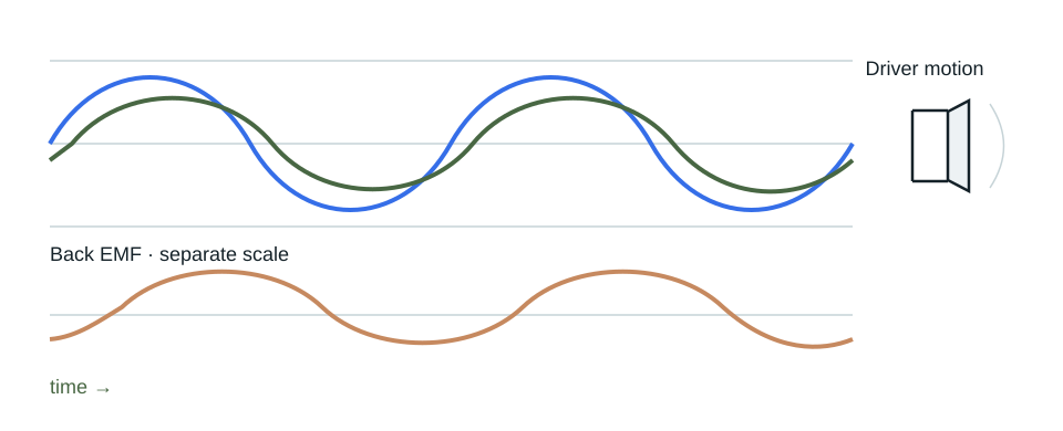
The green current crest follows the blue voltage crest by a small amount.
Illustrative voltage, current and back-EMF relationships, rather than measured amplifier or loudspeaker data.
Select a view to compare the timing of voltage and current, or pause the animation to inspect a moment.
“Before” and “after” describe electrical timing, not when sound reaches the listener.
The important question is whether the amplifier and cable deliver a signal at the loudspeaker terminals that remains close to the one intended. Lower impedance asks for more current; phase shift changes when that current is required. The amplifier’s output stage, power supply and protection circuits determine how it handles those demands, while the cable is part of the electrical path between amplifier and loudspeaker.
To preserve the intended terminal signal, the amplifier must remain stable, supply the required current and voltage, and work with the cable and loudspeaker load. Clipping, current limiting or sufficient cable-related loss changes the signal delivered to the loudspeaker. Audible consequences depend on the size and character of that change and can include distortion on peaks, reduced clean output or altered tonal balance.
Measurements at the loudspeaker terminals reveal how the complete connection behaves under load. Listening comparisons establish the musical significance of the resulting changes.
A fair comparison begins with a defined load, level and test signal. This first test addresses audio-frequency load behaviour; it does not identify an RF path.
A rated watts figure establishes a useful limit under stated test conditions. On its own, it cannot tell us how accurately an amplifier will hold the intended output while impedance, phase and driver motion change. The stronger evidence is behaviour measured into defined loads at relevant levels—not an assumption drawn from cabinet size, amplifier size or a single headline number.
That gives a listener a practical question for a retailer: how does this amplifier behave with this loudspeaker, at the levels I intend to use? A careful listening comparison can then complement the technical evidence without being presented as a substitute for it.
Impedance, phase and driver motion describe important audio-frequency demands. The amplifier–loudspeaker connection also exists at much higher frequencies, where wiring, crossover components and the amplifier’s output network may present different impedances.
High-frequency energy can be present on mains, supply or reference paths, including energy associated with rectification. Protective Earth is an essential safety connection, but it should not be assumed to be a perfectly quiet RF reference. Whether any of this energy reaches the speaker connection depends on the amplifier’s actual circuit and physical layout.
The speaker cable can also couple RF from its surroundings into the connected system. Assessing these high-frequency paths requires a separate investigation from the audio-frequency load test.
An RF carrier can have an amplitude that changes much more slowly than the carrier itself. If a susceptible analogue stage detects that changing envelope, a lower-frequency component can appear at its output. The RF carrier need not lie within the audio band for its modulation to be found there.
In controlled tests of an audio-amplifier circuit, researchers applied RF amplitude-modulated at 1 kHz and measured a 1 kHz output component. Separate op-amp work also reports a response with modulation at 217 Hz. Experiments with RF pulses repeating at 216.7 Hz measured an audio-band response in hearing aids. These results show that the conversion is a measurable circuit behaviour, not merely a theoretical possibility.
These results establish that audio-frequency error can originate in high-frequency exposure. The resulting level depends on the RF strength, coupling path and circuit susceptibility. A complete amplifier–loudspeaker assessment therefore considers both audio-frequency load behaviour and high-frequency immunity.
Quiescent’s own research has found that effects described in the literature also apply within working audio systems. This experience informs our investigation of the amplifier, speaker cable, and loudspeaker as a single connected electrical environment.
High-frequency energy generated within, or conducted into, an amplifier can couple through supply, chassis and reference networks towards its output interface. The cable and loudspeaker provide frequency-dependent paths through which that energy can travel, reflect or dissipate. External RF coupling adds another route into the connection.
Our engineering task is to identify the relevant paths and reduce unwanted interaction with the musical signal. The route and strength of that interaction depend on the amplifier’s circuitry, the cable and loudspeaker, and the surrounding conditions.
During our development and listening evaluations, reducing unwanted disturbance has repeatedly produced a clearer, more stable musical presentation.
Rated power, reactive-load behaviour and high-frequency immunity describe complementary aspects of performance. Together with listening evaluation, they provide a fuller understanding of the amplifier–loudspeaker interface.
Follow the separate questions raised here: what RF can do inside a circuit, how an HF boundary behaves, and how the wider system is connected.
Circuit response
How RF can couple into an analogue circuit and become a lower-frequency error.
Explore RF in Analogue Audio CircuitsMatrix Boundaries
What reflection and transmission mean when an HF path meets a changed impedance.
Explore Return Loss in Audio SystemsWider context
Return to the connected electrical and mechanical view of an audio system.
Explore The Physics of QuietThe load explorer illustrates audio-frequency relationships rather than measured product performance. The cited RF experiments establish conversion to lower-frequency outputs under defined exposure conditions. Quiescent’s research informs the application of these principles to working audio systems; the relevant paths and levels depend on the installation.